Training neural networks with pre-trained models
During my time as a research fellow, I worked on an algebraic reasoning project where we used objects from abstract algebra like rings, ideals and quotient rings to develop models which can reason abstractly to solve Raven’s Progressive Matrices (RPM) questions. For the project, I had to train some object detection and classification models which are used to extract the relevant information from the RPM images for the algebraic reasoning model to reason over and predict the missing patterns.
This post will focus on sharing my first experience and the challenges of training neural networks using pre-trained models. While I had experience with training neural networks, the neural networks were mostly trained from scratch on simple datasets like MNIST. Thus this post serves to document my experience and for anyone who might find the sharing useful. As the algebraic reasoning module is still a work in progress, I will not be mentioning it, except for to solely provide sufficient context for the readers’ understanding.
Background
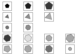
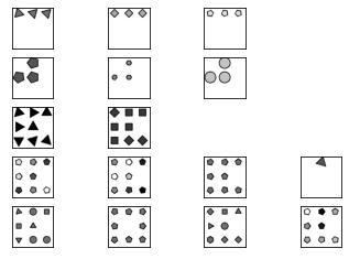
The Raven’s Progressive Matrices is a non-verbal test used to measure general human intelligence and abstract reasoning. Thus they are commonly used to estimate fluid intelligence, the ability to solve problems through thinking abstractly and reasoning, without relying on previously acquired knowledge, of human individuals and now AI models. A typical RPM question provides a participant eight visual geometric patterns, and based on the progression of the patterns, the participant is to identify the missing ninth pattern from a possible eight choices provided as part of the question.


As fluid intelligence does not require any base knowledge, information is solely derived from the RPM images. In the RPM examples provided in Figure 1 above, we can see that each pattern consists of one or more objects which can vary in shape, size, colour and position. Hence the first step is to develop a perception model which simulates how a human participant extracts information from each of the eight patterns, or more generally a model which is able to extract the necessary attributes from each provided pattern. The underlying pattern in the RPM which can be intuitively observed by a human participant to help select the missing pattern, is modelled by an algebraic reasoning module.
While we can build a neural network model from scratch using frameworks like Pytorch or Tensorflow for our perception model, one of the objective of our research was to show the ease of augmenting a neural network model with algebraic reasoning module that will help improve the model. To do so, we made use of publicly available models to develop the perception model, to be then augmented with the algebraic reasoning module. While there are various pre-train models from different developments, the team chose to use the OpenMMLab development for some reasons which I am not aware of.
Data preparation
As a start to test out how effective the pre-trained model will work with our dataset, we focused on how developing an object detection model to detect the shapes of the objects in a single pattern. Although we are using a pre-trained neural network to develop our perception model, there is still a fair bit of work to be done. Using a pre-trained neural network from a particular development would require you to process your data to fit the development’s specification. For the MMDetection object detection toolbox from OpenMMLab, to use a custom dataset for an object detection task, they provide two main options for you to choose from:
- Convert your data to an existing format of COCO or PASCAL
- Convert them to the middle format
Unless your dataset is already in the two popular object detection format of COCO and PASCAL, it can be expensive or tedious to convert your data into those formats. Thus I chose to go with the middle format option which required the bounding boxes annotations to be stored in text files in the following style:
#              // marker to indicate a new entry
000001.jpg     // image file
1280 720       // dimensions of the image 000001.jpg
2              // number of objects in the image
10 20 40 60 1  // bounding box of first object with class 1
20 40 50 60 2  // bounding box of second object with class 2
#
000002.jpg
1280 720
3
50 20 40 60 2
20 40 30 45 2
30 40 50 60 3
The RPM dataset which we used had its own XML annotation format which indicated the position of the objects in the pattern, shape, colour and size of the object as shown in the example:
<Panel>
<Struct name="Singleton">
<Component id="0" name="Grid">
<Layout Number="0" Position="[[0.5, 0.5, 1, 1]]" Uniformity="2" name="Center_Single">
<Entity Angle="3" Color="9" Size="1" Type="3"
bbox="[0.5, 0.5, 1, 1]" mask="[6320,...,47]" real_bbox="[0.475, 0.5, 0.4687, 0.4938]" />
</Layout>
</Component>
</Struct>
</Panel>
In the XML annotation above, the information which we need to train an object detection model using MMDetection are: the bounding boxs of the objects in a pattern and the label of the shape of the objects in the pattern.
This information can be obtained from real_bbox and Type fields of the XML annotation file.
Note that the Type field specifies an integer, which is used to index the shape of the object based on the tuple:
CLASSES = ("none", "triangle", "square", "pentagon", "hexagon", "circle")
Thus a 3 would mean that the shape is a pentagon, as our indexing starts from 0.
While it looks like we could easily parse the XML file to extract the information and append it in a text file as:
#
Image.jpg
160 160
1
0.475 0.5 0.4687 0.4938 3
It turns out that the real_bbox values do not match the format required.
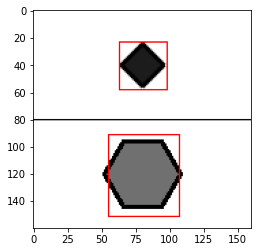
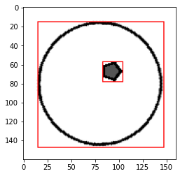
With some trial and error testing, the format of real_bboxes is a perculiar [center_y, center_x, width, height] normalised to a value between 0 and 1, and we need to convert it to the [top_x, top_y, bot_x, bot_y] with coordinates based on the dimensions of the image file as required by the middle format annotation text.
Figuring out the format of the real_bbox was crucial; I could not find any specifications of the real_bbox format and the research assistant which was previously working on this perception module (before it was thrown to me) was encountering NaN errors when she tried to train the object detection model.
Thus the erroneous assumption of [center_x, center_y, width, height] as the real_bbox format could have been the culprit for creating the NaN errors.


With the format clarified, we can write a function that can convert to the format we need for the middle format annotation, and this is the first step of a custom dataset preparation.
Next we need to register our custom dataset within the MMDetection package for it to be recognisable by the package as a dataset.
This registration is for declaring a new custom dataset with your custom specified classes.
As the goal is to train an objection detection model from a pre-trained model, it is very likely that the classes to be detected by the pre-trained model differs from the classes your are trying to detect.
In my case, the pre-trained object detection model was trained on the COCO dataset which has 80 object classes, compared to a mere 6 object shape classes of the RPM dataset, as we saw in the tuple CLASSES.
The custom dataset specification which was required for my model is the Python file (iravenType.py) shown here:
import mmcv
import numpy as np

from .builder import DATASETS
from .custom import CustomDataset

@DATASETS.register_module()
class IRAVENType(CustomDataset):  # name your custom dataset

    # specify your custom classes
    CLASSES = ("none", "triangle", "square", "pentagon", "hexagon", "circle").

    def load_annotations(self, ann_file):
        """

        """
        ann_list = mmcv.list_from_file(ann_file)

        data_infos = []
        for i, ann_line in enumerate(ann_list):
            if ann_line != '#':
                continue
            img_shape = ann_list[i + 2].split(' ')
            width = int(img_shape[0])
            height = int(img_shape[1])
            bbox_number = int(ann_list[i + 3])
            anns = ann_line.split(' ')
            bboxes = []
            labels = []
            for anns in ann_list[i + 4:i + 4 + bbox_number]:
                anns = np.fromstring(anns, sep =' ')
                bboxes.append([float(ann) for ann in anns[:4]])
                labels.append(int(anns[4]))

            data_infos.append(
                        dict(
                            filename=ann_list[i + 1],
                            width=width,
                            height=height,
                            ann=dict(
                                bboxes=np.array(bboxes).astype(np.float32),
                                labels=np.array(labels).astype(np.int64))
                        ))
        return data_infos

    def get_ann_info(self, idx):
        return self.data_infos[idx]['ann']
The functions load_annotations and get_ann_info are functions which are provided by MMDetection.
The needed input is to give your custom dataset a name and specify your custom classes which are indicated in comments in the code above.
With your “registration form” ready, it is now time to register your custom dataset into the MMDetection package.
To register, we need to add iravenType.py to the mmdet/datasets directory.
This directory is found from the location where you have installed the MMDetection package.
If you use a conda environment for your developments, the directory will be located at
/anaconda3/envs/*your_conda_env*/lib/python3.7/site-packages/mmdet/datasets
and within the same directory, make the following additions to the __init__.py file
from .iravenType import IRAVENType

__all__ = [
    'CustomDataset', ... , 'IRAVENType'
          ]
This concludes the registration of my custom dataset IRAVENType which is declared in the iravenType.py “registration form”.
Model retrieval and configuration
The design of MMDetection allows you to retrieve the pre-trained models required from their model zoo using their mim package manager.
If you have followed their installation instructions from the MMDetection page, you will realise that mim provides a unified interface for installing OpenMMLab projects, and accessing the trained models from the model zoo.
The model which I used for the perception module is the Libra RetinaNet objection detection model, and the following is the command to retrieve the model:
mim download mmdet --config libra_retinanet_r50_fpn_1x_coco --dest *dir_to_save_model*
Once the download is completed, you will find the model configuration and trained weights in the form of libra_retinanet_r50_fpn_1x_coco.py and libra_retinanet_r50_fpn_1x_coco_20200205-804d94ce.pth respectively in the directory.
With this you are ready to configure your custom model and fine-tune it on the pre-trained model which we just downloaded.
A configuration of a model allows you to explicitly specify the model and dataset to be used. Here is where you specify the usage of the pre-trained model which you pulled down from the model zoo and also the custom dataset which was registered earlier.
Below is an example of a configuration of a custom model (perception-types.py), with the required or important specifications accompanied by comments for the readers’ further understanding:
# pre-trained model from model zoo
_base_ = '../libra_retinanet_r50_fpn_1x_coco.py'

# usage of custom dataset
dataset_type = 'IRAVENType'

# declaration of specific classes
classes = ('none', 'triangle', 'square', 'pentagon', 'hexagon', 'circle')

data = dict(
    samples_per_gpu=16,    # batch size
    workers_per_gpu=2,
    train=dict(
        type=dataset_type,
        classes=classes,
        # annotation text file for train set
        ann_file='train-types.txt',
        img_prefix='',
        # directory with train images
        data_root = '/local_data/local_data/midformat/rpm-60-20-20/train'),
    val=dict(
        type=dataset_type,
        classes=classes,
        # annotation text file for validation set
        ann_file='val-types.txt',
        img_prefix='',
        # directory with validation images
        data_root = '/local_data/local_data/midformat/rpm-60-20-20/val'),
    test=dict(
        type=dataset_type,
        classes=classes,
        # annotation text file for test set
        ann_file='test-types.txt',
        img_prefix='',
        # directory with test images
        data_root = '/local_data/local_data/midformat/rpm-60-20-20/test'))

model = dict(
    # indicate a new num_class due to new object class
    bbox_head=dict(num_classes=6),
    train_cfg=dict(assigner=dict(min_pos_iou=0.5)),
    test_cfg=dict(score_thr=0.95),
            )
# location of data directory with three folders containing train, val and test samples
data_root = '/local_data/local_data/midformat/rpm-60-20-20'
# pre-trained model weights to be used instead of random initialisation
load_from = "./configs/libra_retinanet_r50_fpn_1x_coco_20200205-804d94ce.pth"
Model training
Finally, we are ready to train the model.
The MMDetection toolbox provides a train.py in the tools folder of its repository.
This Python file can also be found in the installation of the MMDetection package (mmdet), located at ./tools of the mmdetection folder.
As it is too length to call upon the Python file (/anaconda3/envs/*your_conda_env*/lib/python3.7/site-packages/tools/train.py), a copy can be made in your main working directory for convenience.
As I ended up using MMDetection and MMClassification toolkits for the perception module, and their developments both use train.py for training tasks, I renamed them as train-det.py and train-cls.py respectively for my convenience.
Thus the command below is a training job for fine-tuning a pre-trained Libra retinanet model on COCO using my custom configuration perception-types.py for 200 epochs on the GPU with index 0:
python tools/train-det.py \ # can also be test.py to test the mAP or accuracy of model
       ./configs/perception_configs/perception-types.py \ # your custom model configuration
       --cfg-options runner.max_epochs=200 \ # specified to modify configs
       --gpu-ids 0 # gpu to use
Typically the command for sending a training job needs to know the task (train.py or test.py), the configurations of your model.
The --cfg-options allows you to easily change configurations without having to make the edits in the configuration file (perception-types.py), which is especially useful when you are training the same model but would like to vary the batch sizes or epochs.
The --gpu-ids helps to specify which GPU to use so you can submit your job to the GPU with sufficient memory to support your job.
Thoughts
Overall, using a pre-trained model to simplifies the process greatly. A randomly initialised model weights will take a far longer time to converge compared to using model weights which have been previously trained on a huge dataset like COCO. In my case of training an object detection model to detect the objects in a pattern, the shapes of the objects do not have rich features like the objects classes of the COCO dataset. Thus it might be challenging to train a model with reasonable accuracy if we were to train it from scratch. Fine-tuning of the libra retinanet pre-trained model with a mere 6720\(^1\) training samples for 12 epochs (approximately 40 minutes on a single Nvidia V100 GPU) allowed us to obtain a greater than 95% mAP accuracy.
This very first successful object detection model trained from fine-tuning a pre-trained model to detect the various shapes of the objects in a pattern encouraged us to extend it to detection of sizes, colour and position. As the notion of size and colour are less distinct than shape, there were many false positive detections for size and colour. For the positions of the objects, it fared much worst and eventually we tried to use an object classification model to classify the position by first masking all the objects except the object of interest and classifying the image to a position. As I left the team around that time and passed it over to another member of the team, I was not sure how it worked out in the end. But personally, I felt that using an image classification model to infer the position of an object in a pattern is pushing the boundaries of an image classification model; even if the model performs well, we are unable to tell if the model is truly able to understand the notion of position, or is just making the classification based on other patterns or features which we are not aware of.
Overall, the experience was a good one. On the technical side, I learned how to leverage pre-trained models and that data processing is very time consuming. The developers at MMDetection and MMClassification were also very helpful when I raised issues through their Github when I encountered issues; they provided me very timely help and advice which made using their toolkit very much enjoyable. However, their documentation could be further improved; it can be unclear at times and thus required me to do some guessing and trying to get the things working.
This experience also taught me the importance of documentation of your code and eyeballing the dataset.
When I inherited this project, the research assistant only told me how her code ran into the NaN error and showed me numerous versions of her undocumented code with naming conventions which was only understood by her.
Therefore, it was impossible to continue from the code she had and I had to build every thing from scratch.
But this proved to be a blessing; when I started from scratch, I had to examine the data, look at how the labels were stored to fully understand the data which I was to work with.
This is how I managed to find out the reason behind the NaN error due to the wrong assumption of the bounding box format.
This concludes my sharing and I hope you enjoyed the read.
\(^1\): Our initial train-val-test samples consisted of 60-20-20 samples from each figure configuration of the RPM dataset we used. Each RPM question provided a total of 16 patterns, and there were 7 figure configurations, thus giving us \(7*60*16=6720\) training samples in total.